Results of the Fieldtrip & Reflection on the project

Published on 19.09.2026

It was around January, when I finished the DEM-Analysis of my project. Not quite the season to enjoy your time whilst assessing tree health up in the Black Forest, which was why I let that rest until this summer.

I now finally got to do this trip and spent a day biking and counting trees in one of the most beautiful places of this national park.

In this post, you will find the results of the trip and my final thoughts on this project.

Field-trip methodology:

When I wrote the original article, I mainly wanted to validate my finding, that it seemed like north facing slopes were dominated by deciduous trees and south-facing slopes were dominated by conifers. However I ended up, planning my route and sampling spots in a way, so that I could also assess the quality of my clustering.

Quick disclaimer: as this is a hobby project and I was limited by time this trip produced results that aren’t 100% scientifically sound. I mostly wanted to get a feel for whether my ideas might be true and if my system seems to deliver reasonable results. There was no incentive to provide proof beyond a reasonable doubt, which is also why some cluster groups are underrepresented and why the tree counting was performed quite simply.

The sample spots were chosen by me on a map of my route and the latest clustering results (July ‘26) through the most damaged part of the AOI to cover north- and south-facing slopes equally and I distributed them across all cluster groups.

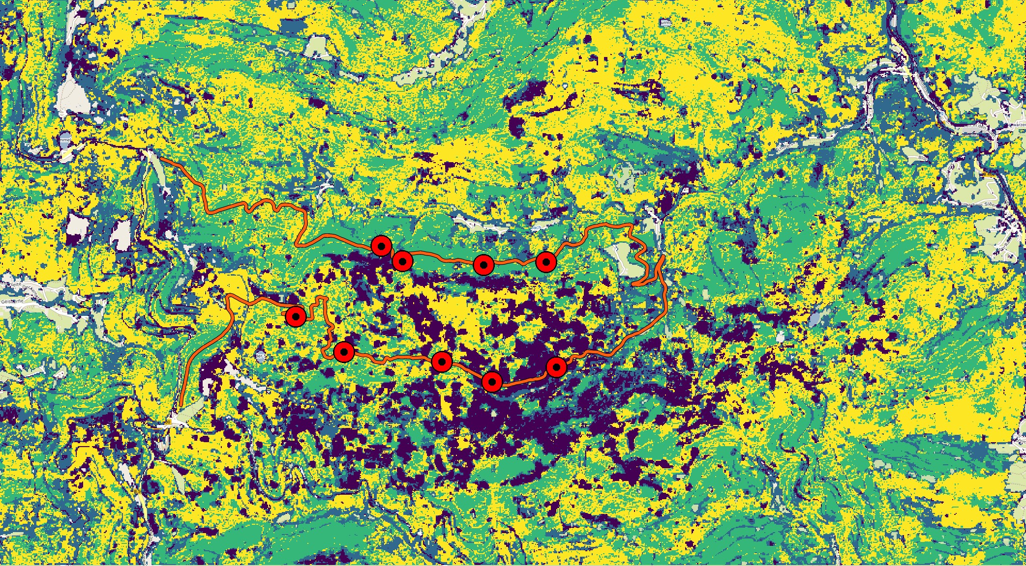
When I arrived at a sample spot, I put my bike aside, walked along the path and counted the trees on one side within a good visibility range until I arrived at 30 counted trees. I classified them with 2 binary features: deciduous vs conifer and alive vs dead.

I chose this absolute number to get a feel for the distribution in a spot rather than tree density, which didn’t align exactly with my goals.

I then took photos of the canopy coverage and the general status of each spot before noting the exact coordinates and continuing to the next one.

Results

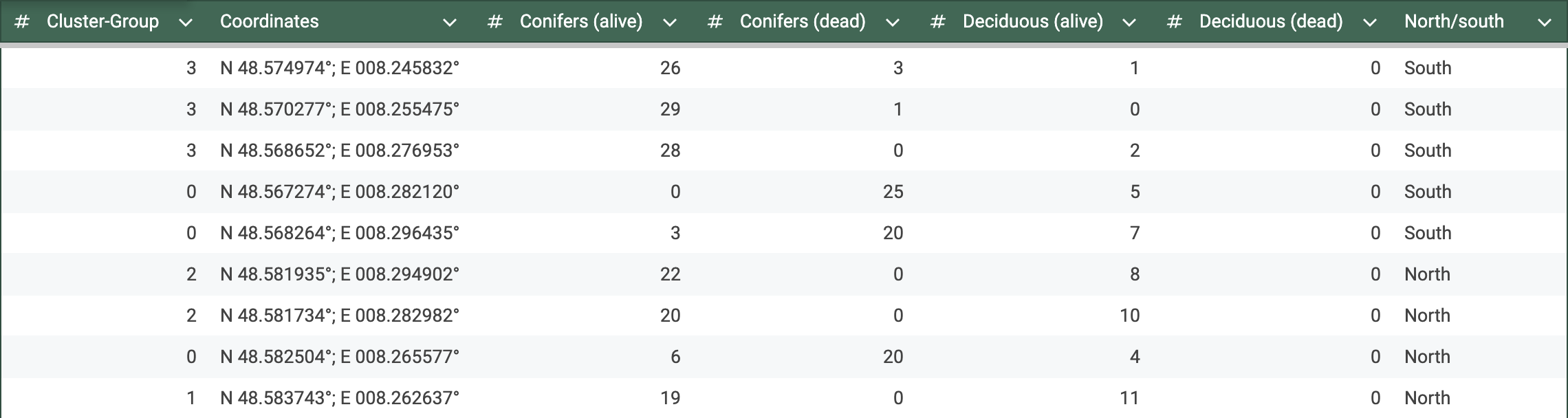
In this table you can see the exact numbers I counted at each spot with the respective cluster group and coordinates.

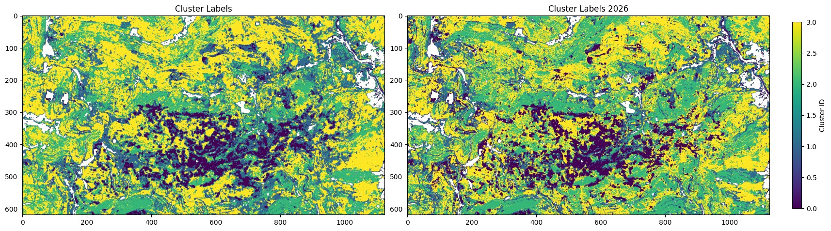
It is easily noticeable that group 1 is only appearing once. This is because when I reran the clustering to choose my sample spots based on current circumstances in the end of July, this group shrunk by a lot, as you can see in the comparison below. This may be due to temporal differences from the first results, which were calculated on data that ended in September or due to randomness in the k-means algorithm.

The following plot shows the mean count per class for every cluster-group and visualizes the main results.

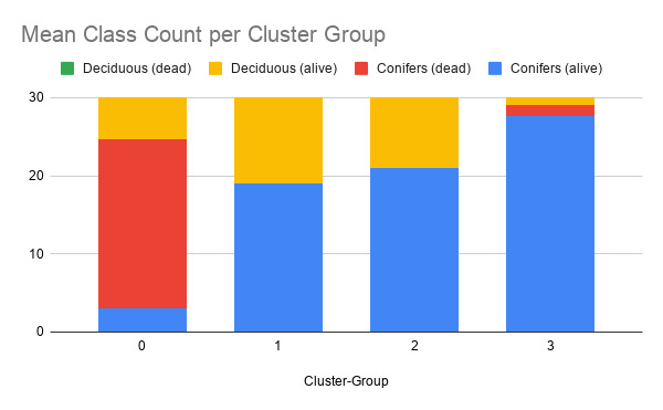
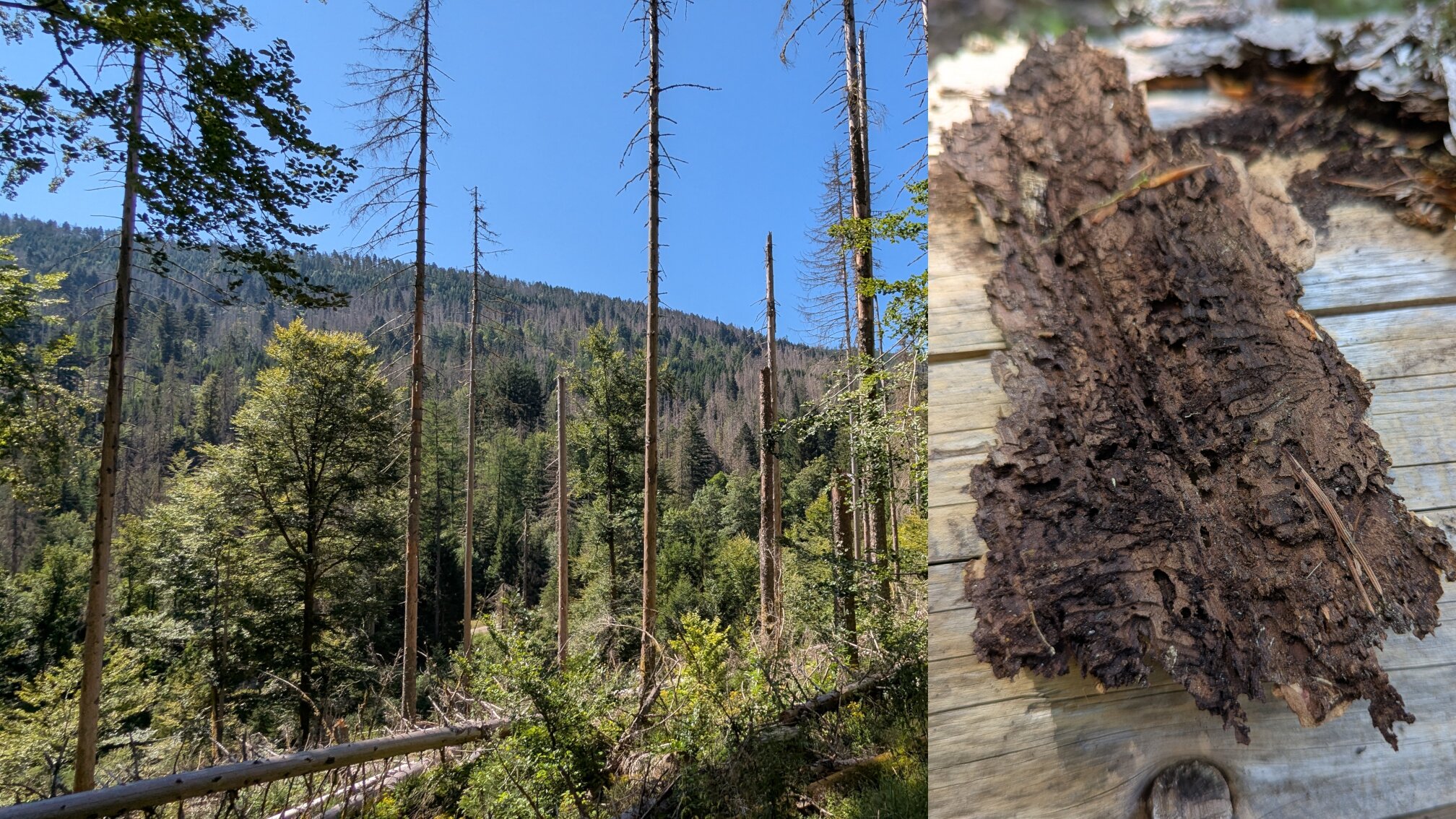
It is visible, how the severely degraded cluster (0) has a notably higher count of dead trees. The quite large difference of this cluster with the others, was also really apparent at those spots: a very high count of fallen and standing-dead conifers, only partly with bark and branches left. However, the deciduous trees in that area seemed untouched. When I picked up the bark of a fallen tree, the small tunnels and grooves made by bark beetles were clearly visible. This suggests that my final conclusion that the degradation was due to bark beetles was correct.

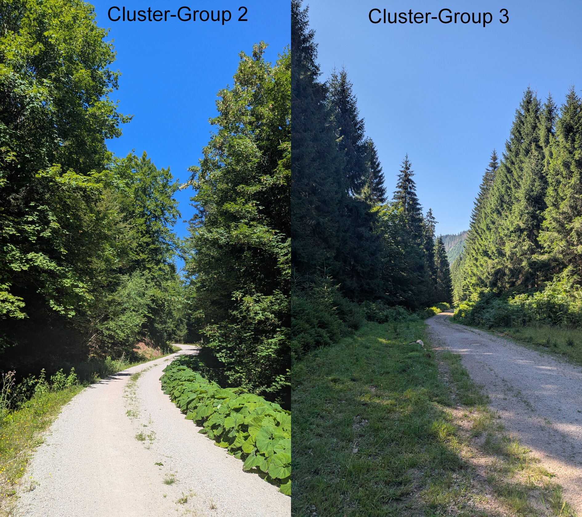
Cluster 2 has a notably higher count of deciduous trees than cluster 3, which suggests that my original motivation for this trip, that the north slopes have fewer evergreen trees, could also be true. Being there in person only reinforces that feeling as the canopy immediately is much denser and has a high share of beech and maple leaves, where as the cluster 3 was almost only made up of evergreen trees.

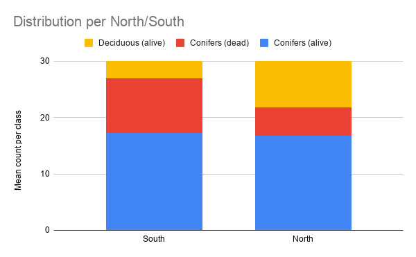
The following visualization shows the mean distribution of tree type per north-/south-slope, which again reinforces the finding, that north-slopes have a higher share of deciduous trees.

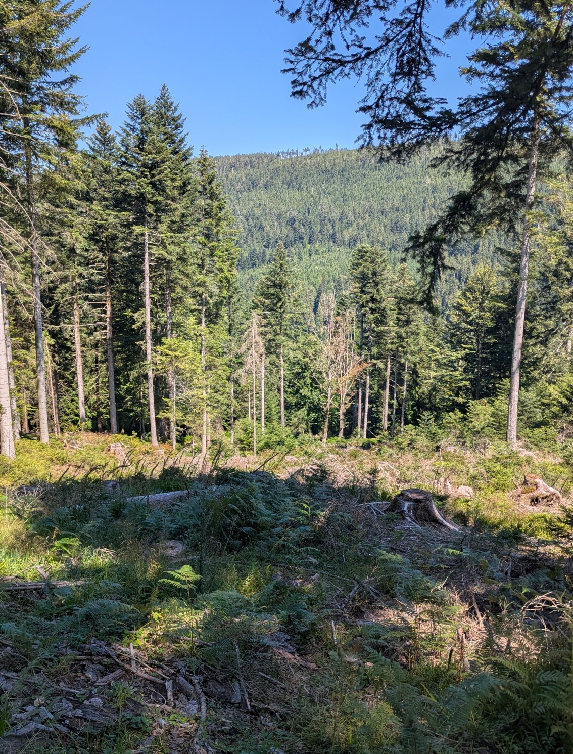
Cluster 1 is generally a bit of a outlier here, as it is based on only one spot. This was due to so few pixels of that group being accessible without leaving the marked paths. On this spot nearly all conifers were cut down in a large sweep, which shifts the distribution.

Thoughts

This project was quite a trip. Just like the tree-counting tour it had its ups and downs and sections, that felt like a dream, next to passages, that felt as if they’d never end.

One could ask the question what stays? What is the final result for me?

From an objective standpoint there is now this code, which allows to perform a distribution analysis of areas with vegetation index features, related to degradation. And that not even really reliable as it is all based around a too simple k-means algorithm. One could even ask, if there are advantages in comparison to a simpler, more interpretable threshold. I’d say so under restrains: it might be less interpretable than hard, hand-picked cuts but this system uses automatically optimized thresholds across combinations of features, which would be really hard to do manually.

From a knowledge standpoint, I reckon there isn’t really anything new. The bark beetle outbreak was very likely known to every forester in that region, as-well as that deciduous trees thrive better on north-facing slopes.

And for me personally?

Overall, I am really quite happy with the result. I learnt a lot and identified many things that I will do differently when I undertake my internship or work on my thesis. First of all, I will document much more thoroughly. I also need to work more scientifically. I deliberately neglected this because I saw it as a hobby project, but now I wish I had done it properly so that it could have formed the basis of my thesis or provided more reliable information.

I would also think beforehand about what the results could and could not say, based on the possible approaches. In this case, I didn't really have much of a choice, but k-means clustering is too random to produce reliable results.

After all, I would talk to people who know much more about the topic in order to make better decisions and take shortcuts. In this case however this would’ve been quite boring, so I am really grateful for figuring it out myself and creating something by myself, that leveraged new knowledge, which I could even “validate” through a small field-trip.

Of course, those were only 9 samples around one mountain ridge. This is no fundament for proper science. However, I wouldn’t consider myself a scientist (at least not yet) and this project was for fun and learnings,

and those I had!